In my last post I talked about the importance of grades being transparent for all stake holders involved. One idea I recommend is having students build their own gradebook in Google Sheets (or any spreadsheet program). This gives them significantly more insight in how grades actually work, behave and gives the student more ownership with their own grades.
However, not all teachers may have the experience or knowledge on how to lead their students to do this – in fact doing it step by step with a class is tough, so I went ahead and made a quick guide.
This guide will help you create your very own functional gradebook so you can keep track of your own grades and have a better understanding of how grades are calculated, figured and how impactful each grade truly is.
How Do I Create A Spreadsheet Of The Assignments And Grades From My Google Classroom?
We will be entering in 20 separate assignments, projects and tests into this sample gradebook. Feel free to add more or less as you see fit.
You want your gradebook to have two halves. The top half will have all the individual assignments. The second half will be the final calculations and final percentage (or grade if you are courageous enough).
Then click the paint bucket button in the toolbar and select the color black. This will make a black line separating the two sections.
Free Gpa Calculator For Excel
I have some done some formatting like centering text, adding a grey background to the cell, increasing the size of the font. Format your gradebook however you like.
*Helpful Tip: You can automatically format the date by selecting the dates and then clicking on Format —> Numer —> More Formats —> More date and time formats*
Now that we have a bunch of data in the top half, we can start to work on some calculations on the bottom half.
Google Sheets Power Tips: How To Use Filters And Slicers
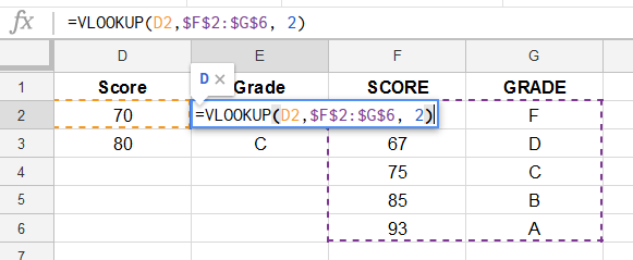
In cell A8 we need to calculate the Total Points. Here we will need to add all the cells in Row 4 – the Possible Points rowThe VLOOKUP Function searches for a value in the leftmost column of a table and then returns a value a specified number of columns to the right from the found value.

The Percentage obtained will be in the first column, while the corresponding Letter Grade will be in the second column. You will notice that the table is sorted from the lowest to the highest grade – this is important as you will see in the next section.
Next, we would type the VLOOKUP Formula where required. In the syntax of the VLOOKUP, after we specify the column to return form the look up, we are then given the opportunity to look for an EXACT match, or an APPROXIMATE match.
Template For Google Sheets
We are therefore going to look up the value in C5 from the range F5:G16 and return the value from the second column. Therefore, when the value is found in column F, the corresponding value in column G will be returned.
Notice that we have used the word TRUE in the last argument of the VLOOKUP – this means that an APPROXIMATE match will be obtained in the lookup. This enables the lookup to find the closest match to 95% contained in C5 – in this case, the 93% stored in F16.

When a VLOOKUP uses the TRUE argument for the match, it starts looking up from the BOTTOM of the table, which is the reason it is so important to have the table sorted from smallest to largest to obtain the correct letter grade.
Aesthetic Google Sheets Templates
As we have used an absolute reference (F4 or the $ sign) for the table – $F$5:$G$16, we can copy this formula down from row 5 to row 10 to obtain the grades for each of the assignments.
The IF Function will also work to get the correct letter Grade for the assignments; however, it will be a much longer formula as you will need to use multiple nested IF statements to obtain the correct grade.
If we want to break the grade down further, as with the VLOOKUP function, we can nest more IF statements into the formula where the IF statement can lookup the letter grade in a corresponding table.

Distance Learning Participation Google Sheet
A weighted average is when assignments on a course differ in the credit value that they count towards the final course mark calculated. For example, during a year, a student may do tutorials, class tests and exams. The exams might count more towards the final mark for the course than the class tests of tutorials.
The weighting column in the example above adds up to the 100% total mark of the course. Each assignment has a weighting assigned to it. To work out the credits received for each assignment, we would need to multiply the percentage received by the weighting of the assignment.
Tut therefore is 4.75% of the 5% weighting available for that assignment. We can then copy that formula down to get the credits received for each of the assignments.
Google Forms Quick Reference Training Card
To see the difference between the weighted average, and the normal average, we can add up the grades received for all the assignments, and then divide these by the number of assignments.

You will notice in the case of this student; the weighted average is lower than the standard average due to his poor performance in Exam 2!
AutoMacro for Excel is an Excel add-in that makes it simple to automate Excel. With a few clicks you can perform complex automation that typically would require programming, you can:

0 Comments
Posting Komentar